A Brief Introduction to Statistics – Part 3 - Statistical Inference

2015/01/04

Statistics

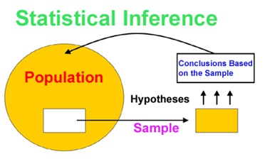
Statistical inference is concerned primarily with understanding the quality of parameter estimates.

Statistical Inference

The sampling distribution represents the distribution of the point estimates based on samples of a ﬁxed size from a certain population. It is useful to think of a particular point estimate as being drawn from such a distribution. Understanding the concept of a sampling distribution is central to understanding statistical inference.

A sample statistic is a point estimate for a population parameter, e.g. the sample mean is used to estimate the population mean. Note that point estimate and sample statistic are synonymous. Recognize that point estimates (such as the sample mean) will vary from one sample to another, and define this variability as sampling variability (sometimes also called sampling variation).

The standard deviation associated with an estimate is called the standard error.
It describes the typical error or uncertainty associated with the estimate. Given n independent observations from a population with standard deviation σ, the standard error of the sample mean is equal to:
SE= σ/sqrt(n)
Note that when the population standard deviation σ is not known (almost always), the standard error SE can be estimated using the sample standard deviation s, so that SE= s/sqrt(n)
A reliable method to ensure sample observations are independent is to conduct a simple random sample consisting of less than 10% of the population.

Difference between standard deviation and standard error
Standard deviation measures the variability in the data, while standard error measures the variability in point estimates from different samples of the same size and from the same population, i.e. measures the sampling variability. When the sample size (n) increases we would expect the sampling variability to decrease.

Confidence Intervals

A plausible range of values for the population parameter is called a conﬁdence interval.
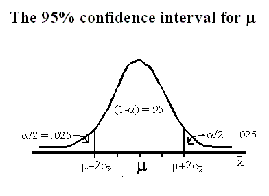
95% confidence interval means, if we took many samples and built a conﬁdence interval from each sample,then about 95% of those intervals would contain the actual mean, µ.

Confidence level is the percentage of random samples which yield confidence intervals that capture the true population parameter.
If the point estimate follows the normal model with standard error SE, then a conﬁdence interval for the population parameter is:
point estimate ± z SE*
where z* corresponds to the conﬁdence level selected.
In a conﬁdence interval, z SE* is called the margin of error (corresponds to half the width of the confidence interval).

Central Limit Theorem
If a sample consists of at least 30 independent observations and the data are not strongly skewed, then the distribution of the sample mean is well approximated by a normal model. Conditions for $\bar{x}$ being nearly normal and SE being accurate:

The sample observations are independent.
The sample size is large: n ≥ 30 is a good rule of thumb.
The distribution of sample observations is not strongly skewed.

The larger the sample size (n), the less important the shape of the distribution becomes, i.e. when n is very large the sampling distribution will be nearly normal regardless of the shape of the population distribution.

Hypothesis Testing Framework
The null hypothesis (H0) often represents either a skeptical perspective or a claim to be tested. The alternative hypothesis (HA) represents an alternative claim under consideration and is often represented by a range of possible parameter values.

Double negatives:
In many statistical explanations, we use double negatives. For instance, we might say that the null hypothesis is not implausible or we failed to reject the null hypothesis. Double negatives are used to communicate that while we are not rejecting a position, we are also not saying it is correct.
Always construct hypotheses about population parameters (e.g. population mean, μ) and not the sample statistics (e.g. sample mean, x'). Note that the population parameter is unknown while the sample statistic is measured using the observed data and hence there is no point in hypothesizing about it.
Define the null value as: the value the parameter is set to equal in the null hypothesis. Note that the alternative hypothesis might be one-sided (μ the null value) or two-sided (μ≠ the null value), and the choice depends on the research question.

p-value:
A conditional probability to quantify the strength of the evidence against the null hypothesis and in favor of the alternative.
The p-value is the probability of observing data at least as favorable to the alternative hypothesis as our current data set, if the null hypothesis is true.
p-value = P(observed or more extreme sample statistic | H0 true)
The p-value quantiﬁes how strongly the data favors HA over H0 .
A small p-value (usually less than signiﬁcance level α < 0.05) corresponds to suﬃcient evidence to reject H0 in favor of HA. Note that we can never “accept” the null hypothesis since the hypothesis testing framework does not allow us to confirm it.

Errors:

The conclusion of a hypothesis test might be erroneous regardless of the decision we make.
A Type 1 error is rejecting the null hypothesis when the null hypothesis is actually true.
A Type 2 error is failing to reject the null hypothesis when the alternative hypothesis is actually true.
Probability of making a Type 1 error is equivalent to the significance level α. Use a smaller α if Type 1 error is relatively riskier. Use a larger α if Type 2 error is relatively riskier.

The Central Limit Theorem states that when the sample size is small, the normal approximation may not be very good. However, as the sample size becomes large, the normal approximation improves.

When to retreat
Statistical tools rely on conditions. When the conditions are not met, these tools are unreliable and drawing conclusions from them is treacherous. These conditions come in two forms:

The individual observations must be independent.
Other conditions focus on sample size and skew.

Veriﬁcation of conditions for statistical tools is always necessary. We need to learn / devise new methods that are appropriate for the data, if conditions are not satisfied. It’s also important to remember that inference tools won’t be helpful when considering data that include unknown biases, such as convenience samples.